3D Stereograms

Glyn Geoghegan

JMC III

Supervisor: Duncan Gillies

Second Marker: Jill Payne

Contents

1. Introduction.................................................................................................................................................

1.1 Abstract.........................................................................................................................................................

1.2 Motivations..................................................................................................................................................

1.3 Applications..................................................................................................................................................

2. Stereo Vision and Stereoscopy.......................................................................................................

2.1 Stereo Vision..................................................................................................................................................

2.2 Dual image stereo viewing..................................................................................................................

Stereo Still Photography....................................................................................................................................

3D Film & TV projection....................................................................................................................................

Computer Generated 3D hollusions.................................................................................................................

Mesh Techniques..................................................................................................................................................

2.3 Theory of dual image viewing...........................................................................................................

2.4 Image Ghosting............................................................................................................................................

3. Stereograms.................................................................................................................................................

3.1 What is a Stereogram?..........................................................................................................................

3.2 Techniques for Generation..................................................................................................................

Depth files..............................................................................................................................................................

The Similar Pixels Technique - the easy way..................................................................................................

3.3 Stereogram Parameters.......................................................................................................................

Depth Parameters................................................................................................................................................

Stereogram Type..................................................................................................................................................

Divergent or Convergent....................................................................................................................................

3.4 Viewing Stereograms...............................................................................................................................

Divergent...............................................................................................................................................................

Convergent............................................................................................................................................................

3.5 Disadvantages of Stereograms.......................................................................................................

Colours..................................................................................................................................................................

Generation Time...................................................................................................................................................

Input Files.............................................................................................................................................................

Useable Depth Levels..........................................................................................................................................

Seeing the @!#* Things!....................................................................................................................................

4. The Repeated Pattern Technique......................................................................................................

4.1 Element Insertion and Deletion.......................................................................................................

4.2 Pattern Substitution..............................................................................................................................

4.3 Full Size Stereograms.............................................................................................................................

4.4 Advanced Ideas...........................................................................................................................................

Shrink-shift effect.................................................................................................................................................

Anti-Aliasing.........................................................................................................................................................

Dual-Direction Stereograms..............................................................................................................................

4.5 References.......................................................................................................................................................

5. Applications..................................................................................................................................................

5.1 Medical Applications..............................................................................................................................

Stereo Research....................................................................................................................................................

Use of RDS in examination of depth perception............................................................................................

Motion perception...............................................................................................................................................

Stereo Technology in General...........................................................................................................................

5.2 Military Applications............................................................................................................................

5.3 Industrial Applications........................................................................................................................

6. Software Design.........................................................................................................................................

6.1 Data Flow Diagrams...............................................................................................................................

6.2 Program Structure..................................................................................................................................

6.3 Algorithm Pseudo Code..........................................................................................................................

Algorithm 1 - Similar Pixels Technique...........................................................................................................

Algorithm 2 - Pattern Deletion and Insertion................................................................................................

6.4 Weird Stuff Algorithms........................................................................................................................

2-Way......................................................................................................................................................................

Dual Level.............................................................................................................................................................

7. Software Implementation & Evolution.....................................................................................

7.1 Prototype Design........................................................................................................................................

Problems Encountered........................................................................................................................................

7.2 Command Line Interface (CLI) design.............................................................................................

7.3 Full Implementation...............................................................................................................................

File Formats..........................................................................................................................................................

8. Conclusions and Future Work.........................................................................................................

8.1 Project Achievements.............................................................................................................................

8.2 Problems and Possible Developments...........................................................................................

9. Software Manual......................................................................................................................................

9.1 Using GJG’s Stereogram Generator.................................................................................................

9.2 User Options...................................................................................................................................................

9.3 Command Line Interface.......................................................................................................................

10. Appendices.....................................................................................................................................................

10.1 Code...................................................................................................................................................................

main.c.....................................................................................................................................................................

stereo.h...................................................................................................................................................................

algs.h......................................................................................................................................................................

algs.c......................................................................................................................................................................

preprocess.c..........................................................................................................................................................

postprocess.c.........................................................................................................................................................

fileio.c.....................................................................................................................................................................

10.2 Figure Legend...............................................................................................................................................

10.3 Some Stereograms...................................................................................................................................

10.4 Acknowledgements...............................................................................................................................

11. Bibliography...............................................................................................................................................

11.1 3D Stereogram............................................................................................................................................

11.2 Stereo Papers..............................................................................................................................................

12. References....................................................................................................................................................

1. Introduction

1.1 Abstract

To investigate and implement 3D Stereogram generation techniques, and to study their applications in real world situations.

This report will outline the various technologies that have been developed to view 3D images from 2D stereo pairs This will include techniques where those pairs are separate sources, such as two photographic slides viewed stereoscopically; or both encoded in one source, such as with stereograms.

The theory of 3D stereograms will be discussed in greater detail, and various techniques for their generation will be discussed, specifically the Repeating Pattern Technique which is used in the software implementation.

Issues relating to the type, quality and style of stereograms will be considered; and problems and solutions relating to this type of 3D illusion will be examined in depth.

A number of medical references to stereo vision in general, and the specific applications and medical thought on random dot stereograms, as well as some military applications have been researched and commented on.

1.2 Motivations

The generation of 3D stereo images from a 2D picture or set of pictures is a fascinating subject, both in the fields of photography and computing. The BBC’s experiments with red/green lens 3D television captured many’s imaginations, Disney’s Viewmaster with it’s 3D photos from films and cartoons intrigued almost everyone who came across it. To this end, this project will cover these various technologies from an aesthetic and technical standpoint.

While on an industrial placement I was given the opportunity to use the Silicon Graphics LCD glasses discussed in Section 0 and I became more interested in the potential of computers in both 3D image generation and processing. As virtual reality head-sets have been developed, the general interest in 3D technologies has been heightened, and the rise of stereograms is symptomatic of this.

Stereograms have gained popularity, since they first became prominent in poster shops around the country in the early 90’s, and due to the Magic Eye and other series of books containing stereograms. This explosion in popularity encouraged a friend and I to devise the generation technique listed later as The Similar Pixels Technique last year. This project has provided the opportunity to spend more time investigating stereo-technologies and their applications for this project, and to devise a more versatile and powerful set of algorithms for generating Random Dot and Colourfield Stereograms.

1.3 Applications

As mentioned in the abstract, there are a number of applications of 3D stereo technology, ranging from entertainment and leisure, to practical applications in commercial industry, chemistry and medicine. These are discussed in detail in the later chapters, chapter

2. Stereo Vision and Stereoscopy

Stereo vision in human beings is possible because of natures positioning of the two eyes in a forward facing position. This allows the brain to receive two slightly different views of the world, and from the slight discrepancies in these two views, resolve 3D depth information of the perceived objects. Homo-sapiens is one of only a select few animals capable of 3D vision. Birds, reptiles and most other mammals have their eyes positioned on the side of the head, for greater vision of their surroundings, but this precludes 3D perception as we understand it.

This perception of the 3D world can be simulated in two dimensions to create an illusion of depth, by feeding subtly different images to each eye from a 2D source, and a number of ways have been devised to provide these separate 2D sources, which will be discussed later.

First, however, it is useful to discuss how 3D vision works, and the changes in the eye as it views objects at different depths.

2.1 Stereo Vision

Shown below is an illustration of the angle of vision of the eyes when viewing objects in 3D. The first shows the eyes focusing on a far object; the plane of focus is distant, and the angle a is small. When the object is close, as in the second case, the plane of focus is nearer, and the angle a is larger.

Figure 2-1: Depth Perception

The objects at different depths are projected through the lenses of the eye onto different parts of the retina. The brain then calculates the depth of the object from the differences between these two projected images; when an object is near, there is a large difference and as the object moves farther away, this discrepancy is reduced until the object is at infinity (practically greater than 30 feet away) when the images on the left and right retina are identical.

Since the important factor in stereo vision is the difference between the scenes projected onto the left and right retina; by providing these images directly to each eye, rather than letting the eyes as a pair perceive the different depths of objects, we can simulate the 3D effect.

2.2 Dual image stereo viewing

Many different ways of providing these dual images have been devised, for use on both still and moving images, and using one or two source images.

Stereo Still Photography

Stereoscopic still-cameras, which take two photos simultaneously through lenses separated by approximately the same distance as the human eyes have been popular in various guises over the years. Many people are familiar with a common childhood toy, the 3D Viewmaster.

3D Viewmaster

Made popular by Disney, the 3D Viewmaster is a binocular device which takes changeable cardboard discs, with the two stereo photographs on opposite sides of the disc. These opposing images are then viewed through the eye-pieces, feeding the different images to the left and right eyes.

Figure 2-2: Binocular systems - the 3D Viewmaster

This technique gives full-colour, photograph quality 3D images, but is hampered by the necessity for the Viewmaster, the 3D images cannot be viewed without this extra equipment.

This type of technology has been used in simpler forms since the early days of photography. Mounting the two stereo images on a stand so that they are placed directly in front of the eyes can be just as effective, the Viewmaster simply provides a more definite separation; the left eye cannot see the right eye’s image and vice versa.

Namco

One camera manufacturer has designed a photographic and development processes allowing stereo images to be taken and printed into a single photograph, viewed without any other special equipment, but I have been unable to find out further details.

3D Film & TV projection

The movie industry has toyed with a number of gimmick’s over the years, moving seating, smell-o-rama and, of course, 3D. The popularity of 3D films, however, has been limited, as it is more expensive to produce a 3D film, and the technology for viewing the end result has it’s limitations and side effects.

Colour Filters

One common technique, used on both film and television, is that of red/green or red/blue colour separation. This allows both of the stereoscopic images necessary for 3D viewing to be present on the same source, and by use of colour filters; the images can be directed to the individual eyes.

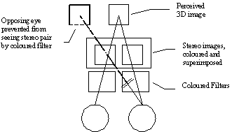
Figure 2-3: Colour filter image separation

This technique allows viewing of the 3D image by use of coloured filters over the left and right eyes. However, the colour information is generally lost, as colour in the stereo images interferes with the filtering. The separation of the images is generally inadequate, causing a blurring of the 3D effect, and usually gives the viewer a headache after a short period.

Plane Polarisation

This is another technique used in cinema, to greater effect (especially in the film Jaws 3D). This time, two projectors are used, each sending one of the stereo sequences to the screen. The isolation of the two images is achieved by polarising them at 90^o to each other. The glasses worn by the viewer, rather than being different colours, are polarising filters offset by 90^o, one vertical and one horizontal.

This allows full colour information to be retained, but the viewer must keep the lenses lined up accurately with the screen, as any angular deviation will pollute the images reaching the eyes, and again cause a blurring effect.

Plane polarisation can only be achieved with projected; not broadcast (TV) or print media, as the source images also have to be polarised and projected over each other.

Computer Generated 3D hollusions

Although the impact has worn off slightly now, computer technology has been quick to embrace 3D technology. Computers are ideal for generating any still or animated 3D system, due to their ability to calculate the complex equations commonly associated with 3D technology at a great speed.

Virtual Reality

Virtual reality is a field under continuous development. It is now common in both entertainment arcades and the home market to see the Virtuality brand of VR headset; available on a number of consoles. It uses a technique similar to the Viewmaster mentioned earlier, by supplying the left and right stereo images to the eyes through small LCD screens mounted in a headset. This headset also feeds directional information back to the software generating the stereo images, allowing the user to look around a virtual world in full 3D. The speed of the systems using this technology at the moment severely restricts the quality and speed of the 3D world the user is subjected to, although this technology is, needless to say, improving constantly.

Computer controlled LCD goggles

Another technique, used especially in Silicon Graphics computer systems, again uses computer controlled goggles. This time, however, the system is continually alternating between the two stereo images on screen, and the isolation of the left and right source images is left to the headset.

The computer synchronises the goggles by using transparent LCD windows in the glasses, which can individually made opaque by applying a current to the crystals. At any moment in time, only one of the eyes can see through the goggles, and this is synchronised to the image currently being displayed on screen.

This has the advantage that the image quality is higher than with the VR headset systems, as any full-size, high quality monitor can be used; rather than a 2” low-resolution LCD screen - although the processing power required to generate a full-screen 3D image is much higher than the smaller LCD version.

This SGI system is used to good effect in commercial chemistry, where it is useful in fields such as organic chemistry, where large and complex organic molecules can be generated and viewed in 3D.

Mesh Techniques

By placing a mesh in front of a 2D image, the eyes can be prevented from looking at the opposite eye’s component of the 3D stereo pair. This allows the images to be separated in much the same way as the masking plate in a CRT allows the guns of the tube to generate a TV picture.

Figure 2-4: Mesh image separation

The complexity in constructing the mesh, and in generating the associated 2D image, makes this type of stereo image quite rare, and I have been unable to find any examples.

2.3 Theory of dual image viewing

All of the above techniques rely on having a 2D image presented to the eyes, containing the information necessary for the brain to perceive the full 3D image. In divergent viewing, this 2D image will be between the eyes and the plane of the 3D scene. (It is called divergent viewing as the eyes must diverge to focus beyond the plane of the 2D image. You can refer to Figure 2-1 to see why the eyes are more diverged when looking at a distant object).

We can trick the brain into thinking it is looking at a more distant object than it is, by introducing a stereo pair

Figure 2-5: Divergent stereo image viewing

The image the individual eyes are receiving is simply the square, the brain still perceives the object to be just one square, at the original depth, as the plane of focus of the eyes is still at this greater depth. So by introducing the 2D image at the intermediate depth, we have retained the perception of an object at a greater depth.

This illustration shows divergent 3D viewing, one can also perceive 3D through convergent or cross-eyed viewing, and this will be discussed later.

The artificial 2D depth image is completely blocking the eyes view of the original, distant object, which we can therefore remove. This means that the brain is now perceiving a totally artificial object which it has created from two images placed before the eyes. The depth of the perceived object is governed by the separation of the matching parts of the superimposed images.

Below we see a series of lines which the eyes have focused beyond, creating a ‘base depth’ for the 3D hollusion.

Figure 2-6: Perception of apparent depth from a repeated pattern

As before, the plane of focus is beyond that of the 2D image, and the brain perceives the depth of the repeated pattern to be farther away. If we now introduce another repeated pattern, but with a greater separation, the brain sees these objects at a different depth (Figure 2-7).

Figure 2-7: Multiple depth levels from different spacing

We can see from his picture that the greater separation of the dots compared to the lines, causes the brain to calculate their 3D position to be further away than the lines. The natural reaction of a viewer at this time would be to re-focus the eyes to the nearer plane of the paper, seeing simply a row of dots and lines, but if the eye’s focus is forced to remain behind the 2D image, the 3D effect should be clearly visible.

The following figure is a correctly scaled version of the above example. By diverging or converging (crossing) ones eyes such that the vertical lines separate horizontally, and then re-converge out of phase, they should appear to be a slightly different depth to the page, and due to the different displacement of the dots, they should appear to be at a different 3D depth to both this page and the lines, either behind the vertical lines (if viewed divergently) or in front, (if one has gone cross-eyed).

The cross-eyed effect is the easiest to achieve; by holding ones finger approximately 2 inches in front of the paper and focusing on it, you should see the lines and dots on the page separate. Move the finger slowly back and forth until the dots and lines match, and you should be able to remove the finger and see the 3D depth effect.

There will be a fuller discussion of how to view these types of 3D image later, so don’t dwell to long on trying to see the effect, unless you wish to check the previous information on stereoscopy is true!

Figure 2-8: Multi-depth level example

Similarly, if the following example is viewed con- or divergently, due to the varying separation of the word stereo the lines appear to be at different depths.

STEREO STEREO STEREO STEREO STEREO

Figure 2-9: Differing depths through text spacing

Again, the below stereo pair produces a 3D image, which, as the two images are slightly distorted from being proper cubes, appears to be a real (although transparent!) 3D object when viewed stereoscopically.

Figure 2-10: 3D object from two perspectives

Our final illusion is a development from the variable spacing pictures shown previously. We can vary the inter object spacing along just one line of base images, rather than having different lines of the image at different depths. This gives an apparent variation in depth across a single line of objects, rather than simply different lines in an illusion being at different 3D levels.

Figure 2-11: Smiley Faces

This method of varying the spacing between similar points in a line of repeated patterns forms the basis for the stereogram generation technique outlined later in this report. It should also be noted from the above examples that, due to the positioning of the eyes in a horizontal line, the 3D effect is dependant only on object spacing within a single row; there is no link between separate rows.

This statement can be tested by viewing, for example, Figure 2-9 stereoscopically, and then slowly turning tilting ones head. The dots will soon break back into their stereo pairs as the eyes are moved away from the horizontal, and the stereo effect will be lost.

2.4 Image Ghosting

It is clear from attempting to view the above images that this is not the best way to see a 3D image. You will probably have noticed that as well as the desired 3D object, there are two ghost images, the two elements of the stereo pair (especially visible with the 3D cube, Figure 2-10).

This undesirable effect is caused by one eye seeing some of the information that should only be privy to the other eye. This can be illustrate as follows:

Figure 2-12: Ghost images

If the component images in the 3D plane are readily identifiable in the 2D source image, the brain will visualise ghost images off to the sides of the correct 3D projection. To avoid this, we must find a way to link the corresponding sections of the stereo images in such a way that these link points are only identifiable as such when the source is viewed as a stereo-image.

We have seen how various 3D techniques isolate the left and right eye’s images, but all of the techniques so far require the use of equipment, be it red and green glasses or a Viewmaster. We ideally want to find a way to encode the 3D data into a simple 2D picture, without the need for any other apparatus.

This is where we finally reach the 3D image type the project is primarily concerned with, that of the Random-Dot and Colourfield Stereogram. These 3D hollusions can be viewed directly off the page, with only a small amount of training of the eye and brain (although seeing one’s first stereogram is usually a difficult task - the results are more than compensatory!)

3. Stereograms

3.1 What is a Stereogram?

We have already discussed the various ways that 3D technologies have of supplying the stereo image pairs to the viewers eyes, and stereograms simply introduce another way of encoding these two images into one planar picture.

A stereogram may simply be a seemingly random picture, containing a series of coloured dots (a Random Dot Stereogram) or it could be some kind of repeated pattern, strangely distorted across the page (a Colourfield Stereogram). Either way, these images form both a pleasing 2D abstract picture, and when viewed correctly, a 3D depth illusion.

The trick is that the seemingly random patterns, or the repeated distorted image in the 2D picture have, in fact, been carefully generated, applying the concepts discussed in the following chapters.

3.2 Techniques for Generation

It us useful at this point to recap on some of the phenomena we have noticed from our investigation into 3D technologies.

· The brain is the most important factor in determining depth within a perceived scene. The eyes simply provide the brain with the information necessary to derive this 3D information. The eyes can be given the relevant information in any we choose.

· The most important aspect of faking depth information is the variation of the distance between similar objects across a row of the eyes field of vision. Any perceived depth is created across the columns (or x co-ordinates) of a y-plane line of a scene, and there is no 3D interaction between different rows (or y co-ordinates).

· For this 3D illusion to work, each eye must see a separate, but identical representation of each point of an object, spaced to create the 3D depth.

If we consider these factors in a 3D scene; with an object, the 2D plane containing the stereogram, and the viewers eyes (Figure 3-1), we can examine the geometry required to generate this illusion.

Figure 3-1: A 3D Scene

If we first take one point on the object, we can see that we first need to trace a line from it’s location in 3D, through the 2D plane to the left eye. If we set this screen pixel to a colour, we must then also trace a ray from the same point on the object to the right eye, and set the intersected 2D pixel to the same colour.

If we now consider that, rather than starting from a point on the object, and rather consider a ray from the left eye through each point on the 2D plane and it’s intersections with either an object defined in 3D space, or some pre-defined backdrop, set behind all of the objects in the scene, we can derive am algorithm to calculate a 3D stereogram from co-ordinate scene information:

main

{

clear screen to white

for each row y

for each column x

if the pixel x, y is white

{

pick a non-white colour

call tracepoint(x, y, colour)

}

The tracepoint algorithm is where the hard work occurs;

tracepoint(x, y, colour)

{

repeat

setpixel (x, y, colour)

trace a line from lefteye(x, y, z) through (x, y, plane_of_z)

calculate the co-ord of the nearest point in 3D of either an object or the backdrop on the line

trace a line from this point to righteye(x, y, z) and calculate the intersection with the 2D plane

if there are no nearer objects to the intersection

set this intersection point to colour

else

break

set x to this new intersection points x co-ord

until x > screen width

}

The algorithm scans across each line of the scene setting linked pixels; (that is, pixels which the eyes must look through to create a depth point in the 3D plane), to be the same colour.

The algorithm is incomplete, (there is no discussion of the co-ordinate geometry required to perform this task) but is does give a general idea of how this type of technique works.

In the tracepoint routine, there is some elementary checking to make sure that since the eyes will look through the same 2D point to objects at various depths, that the nearest to the eyes (and therefore the one they would actually see) is the object that is projected into the stereogram. Again, though, this checking is passed over in simple terms in the algorithm as, thankfully, there is a faster and cleverer way of calculating the scene information.

There is a fuller discussion of the co-ordinate technique in PCW, December 1994[i].

Depth files

The largest step is simplifying the generation is to remove the complex full 3D representation of a scene (such as that given to ray-tracing software) and replace it with a 2D mock-up of the real 3D world. The common 2D solution is to have a series of objects drawn with their colour signifying their depth in the 3D scene (black being the farthest point, the backdrop; white being the nearest - the plane of the page; and the various greys the depths in-between). This immediately removes the need for calculating depths of objects (near objects automatically obscure far ones), and we can simply scan across this depth file for the information necessary to create the illusion.

It should be noted, however, that more care must be taken over drawing this depth file; the user must consider the depths of the objects they are drawing before committing them to the scene.

The Similar Pixels Technique - the easy way

Now we have developed the concept of a depth file, we can consider a simplification of the co-ordinate technique, which I have called the similar-pixels technique. The algorithm for this is considered in detail in chapter 0, as it is the basis for one of the generation techniques used in the first software prototype, but I will describe the theory of this idea here.

If we again consider the recurring theme that the eyes must look through 2-points to perceive a third 3D point with depth, and couple this with the fact that we are now generating a stereogram from a scene which effective contains an array of pixels, with their respective depths, we can immediately see that our job has been made a lot easier.

If we consider each point across the line in turn, allocating it a colour (if it hasn’t already been given one by a 3D partner), and then determine it’s linked-neighbour (which we can easily do using a function of it’s horizontal x-position, and it’s colour/depth) we can set it’s partner to the same colour.

For example, if we are somewhere along the line, considering a point which has been coloured ‘red’ we would take it’s depth (say 55) apply a function to it; (since black is generally considered to be colour 0, and we have set this to be the farthest point; our function will return white (255) - depth; in this case, returning ‘200’); we would set the pixel 200 places to it’s right to red. We would then consider the next pixel, and set the pixel 255-depth to it’s right to it’s colour etc. until we have linked every pixel in the file to it’s neighbour.

Once we have passed across each line of the depth file, linking the pixels in this way, we should have compiled a complete stereogram, holding all of the depth information necessary for viewing the scene described in the depth file. Each pixel is now the same colour as it’s linked neighbour, but due to the random choice of new colour each time a non-linked pixel is processed, this linking information is hidden from the viewer until they view the stereogram properly - it appears to be a random pattern.

As with most computer-procedures; this technique is best described using pseudo-code, and it may be useful at this point to refer to section 0 for a fuller understanding of the concepts involved.

The similar pixels technique is probably the simplest way to generate a stereogram, but as with most simple solutions, there are drawbacks. It is not very versatile, making it difficult to adjust the many parameters that can make a good, easily viewable or impressive stereogram.

These factors are integral to the technique used in my implementation, which takes the inter-pixel spacing within the stereogram to be the most important factor, taking a pattern and varying the width of this repeated pattern to encode the depth information.

I have called this generation idea the Repeated Pattern Technique, and it is discussed in detail in Chapter 4.

Before we move onto this technique, it is useful to consider the parameters effecting stereogram generation, and some of the associated problems.

3.3 Stereogram Parameters

There are various ways the output from a stereogram generator can be changed. The most important factor is that of the number of depth-levels possible in an image. We must also consider the type of 2D image; random dot or colourfield, and whether the stereogram is to be viewed divergently or convergently.

Depth Parameters

Since the depth levels in a stereogram are determined by changing the distance between the similar pixels, there is some quantisation of the number of apparent depth levels in the image. The numbers of levels of depth should be as high as possible to allow realistic, smooth edges to be produced on objects which make use of the z-plane. Lines in the x and y directions are as smooth as the resolution of the output device will allow, and are to all intent and purpose, infinitely variable.

The number of depth levels in an image, the dpi of the output device and the width of the repeating pattern. These three elements are linked by the simple equation

DPI of Output Device

Although this factor is determined by the output device itself, it is important to be able to vary it. Commonly monitors will have a dpi of somewhere between 72 (for a 14” 1024x768 display) and 128 (16” 1280x1024 display), so with a pattern width of somewhere between 1 and 2 inches, we have a depth-level range of between 72 and 256. On a printed output, however, where the dpi is much greater (300 or 600 dpi), at the same widths we can obtain between 300 and 1200 depth levels, allowing for a much smoother 3D image.

Pattern Width

As the pattern width is increased, the possible number of depth levels correspondingly increases. This, however, has it’s boundaries, as the pattern must be wide enough for the eyes to lock-on to the stereo image, and it must be narrow enough so that the eyes can diverge enough to overlap the repeated pattern.

The pattern must be narrower than the distance between the eyes (as shown below) and the closer it gets to this width, the harder it is to view.

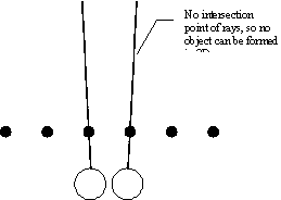
Figure 3-2: Non-convergence due to high pattern width

Due to the eye’s ability to cross almost completely, there is no such upper restriction on pattern width with convergent stereograms.

dpi and pattern width contrasted

The following table compares the effect of increasing the number of depth levels by increasing either the pattern width or the output device dpi.

	Pattern Width	dpi of output device
Effect on apparent depth	Due to the increased amount the eyes must diverge, the perceived distance of furthest point increase, thus increasing the apparent depth	Since the eyes are still focusing on the same point beyond the plane of the 2D image, there is no increase in apparent depth
Effect on image smoothness	The inter-level distance is unaffected, there are just more levels introduced, so there a reduction in image smoothness, due to the increase in perceived maximum depth	Due to the increased resolution, more levels can be included in a smaller area, so the inter-level distance is reduced, increasing the smoothness of the image

So for the ideal stereogram, we need a high resolution output device, and a large pattern width (and therefore an experienced viewer!), allowing the image to contain both a large perceived depth, with smooth depth grading between the viewer and the furthest point.

Stereogram Type

The apparent smoothness of a stereogram is also effected by the type of stereogram generated. At all stages of 3D perception, the brain plays a vital role in how the image is presented to us, and this effect can be maximised by the type of the 2D image presented to the viewer.

If there is a repeated pattern on the 2D stereogram, such a persons face, or a tileable pattern (in the colourfield variants) or a bias in the random pattern (say, 70% white rather than 50/50 white/black), the brain will interpolate the discrepancies in the staggering of depth and produce a clearer image.

This can be seen by generating two stereograms, one RDS and one Colourfield, from the same depth file with the same parameters. The brain will smooth the ledges out of the colourfield file far more effectively than in the RDS.

This effect is illustrated by Figures 10-1 and 10-2 in the appendix.

Divergent or Convergent

As mentioned earlier, a stereogram can either be viewed divergently, or convergently or cross-eyed. Any stereogram can be viewed either way, but for the best results, it must be generated with a type of viewing in mind.

By viewing a divergent stereogram convergently, a peculiar effect is achieved in that the objects which should rise from a distant plane toward the viewer are now inverted; disappearing away from the viewer from a near point into the plane of the paper. Similarly, pits in the stereogram now become raised regions.

A convergent stereogram can easily be generated, by either the user or the software inverting the original depth map so that when it is processed, the output stereogram has already been inverted for convergent viewing.

By again viewing Figure 10-2 again, divergently, we can see this unusual inversion effect. Figure 10-3 is a stereogram created from an inverted version of the same depth file, and can be viewed correctly by crossing one’s eyes.

3.4 Viewing Stereograms

Divergent

The biggest drawback of stereogram technology is how hard it is to initially view one (although with practice, it becomes incredibly easy); and the difficulty involved in explaining to someone how to view one - which I will now attempt to do.

The are a number of ways to aid viewing, and the trick is to find a way that works and keep trying, until you have sufficiently trained the eyes to diverge, relax and look beyond the page; while you concentrate on the image forming before you.

First we’ll consider viewing techniques.

· If the stereogram is on a monitor screen, or is printed and displayed behind glass (or any reflective surface); by staring at one’s reflection on the surface, the eyes are naturally focusing beyond the plane of the page, and you should therefore be able to see the 3D illusion (by moving one’s head slowly back and forth in front of the screen, while still looking at the reflection, you will change the amount the eyes have been diverged, and should therefore be able to catch the stereogram)

· If one holds the stereogram directly in front of the nose, and then moves it slowly away - while trying not to refocus the eyes on the page, when the stereogram is about one foot from the face, it should become visible. Again, by varying the distance slightly as you start to see the image, it should come clearly into focus

Those are two quick ways to try and view stereograms, and if they are repeated viewed in this way; the eyes should become used to relaxing into seeing stereograms, but there are some better ways to train the eyes.

· The first is an old trick: Hold your two index fingers tip to tip at the bridge of your nose (so that the two fingers are in a straight line, pointing at each other) Now, as the hands are moved slowly away, a third phantom finger; with nails at both ends, forms due to the discrepancies in the image the two eyes see.

When the fingers are moved away from the face, if you do see the third finger, then you are viewing divergently; your plane of focus is far beyond your fingers.

· Similarly, if you just hold one finger vertically in front of the nose, and slowly move it away while focusing on a distant object (for example the wall of the room) you should be able to see two fingers side by side.

· With either of the above two techniques, if you can then move your hand so it is directly in front of a stereogram, without changing your plane of focus (so you can still see the phantom finger, or two fingers side by side) - with a bit of luck and maybe a little work in focusing the eyes, you should be able to see the stereogram.

The important thing to remember is that you must look through the page; the eyes must focus beyond the stereogram, and as this happens, patterns on the stereogram will break up and overlap, and eventually they will again overlap, but slightly out of phase; allowing the 3D information to be perceived.

My Viewing Aid

On the stereograms generated by my software, there are two small dots printed on the final image at the top of the page

As you stare at the stereogram, relax your eyes so that the two dots appear to become four (using any of the aforementioned techniques may help at this point)

As you relax you eyes, the dots should slowly converge....

And eventually become 3 dots....

At this point, since the dots are spaced at the same width as the pattern width, the stereogram should be visible. So, if you look slowly downward (concentrating on keeping the three dots overlapped) you should see the stereogram burst into life!

When viewing stereograms, you should concentrate on diverging the eyes; not on the 2D surface image (which will look strange as the pattern is diverged). When you have diverged your eyes the correct distance, the pattern will again look normal - although now it will be covering a 3D scene, rather than a simple 2D surface.

Convergent

Convergent or Cross-eyed stereograms work on a similar technique, but can have a far more striking effect. With this type, the 3D image is formed between the viewer and the 2D plane, creating a holographic-type effect that the viewer often feels they can reach out and touch.

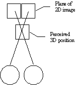
Figure 3-3: Divergent image viewing

Unlike divergent viewing, where the eye is relaxed, with convergent viewing the eye-muscles are contracted, and as such there is eye-strain associated with cross-eyed viewing.

Many people find it easier to cross their eyes and near-focus, than to focus beyond the plane as is required with divergent stereograms.

By holding one’s finger approximately 2” (depending on the parameters used to generate the stereogram) between the plane of the 2D image and focusing on that, the 3D image should become visible. If not, then by slowly moving the finger back and forth, the scene should come into focus.

3.5 Disadvantages of Stereograms

Colours

Through our examination of stereograms and their generation, we know have a fairly good idea of the physical makeup of these 3D illusions; and from this we can examine their biggest problem.

Stereograms don’t contain proper colour information

As we have seen when viewing them, whatever the pattern is that contains the 3D information, be it random dots, psychedelic patterns or someone’s grinning face, when the 3D illusion is viewed, that same pattern is present all over the scene.

This is a necessary part of stereogram construction; we have seen from the previous discussion that the stereogram works by providing pairs of identically coloured pixels to the viewers left and right eyes, so we are forced to colour a whole series of pixels across the page in the same way. Although the initial choice of colour is ours, the placement of objects in the 3D world determines the colours used further along the line.

Consider the scene below:

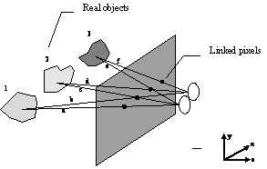
Figure 3-4: Determining pixel colouration

If we consider that the leftmost of the 4 linked pixels has had it’s colour determined by object 1 (ray a), we can see that it’s linked neighbour, (traced with ray b), the next pixel to the right, also has to have this colour (as the right and left eyes must see the same point).

This is fine; the eyes will now perceive that point on object 1 to be the correct colour. But now we have the problem that ray c traced from the left eye through the point just coloured for the right eye intersects with object 2. We can’t change the colour of this pixel to match the second object, as it is already linked to the first object.

This then has the knock on effect that the right-eye pairing for this pixel (the third dot across in Figure 3-4 - by ray d) must also be the same colour; and so on across the whole line: Rays e and f cause the fourth point to be set to the same colour.

Further more, so that the brain is given enough unique pairing information to decode the 3D scene, we must use as many different colours as we can, to isolate the various pairings of pixels in the image. This means that, ideally, the pixels adjacent to the one we first traced our ray through should have distinct colours; so they cannot share object 1’s colour, even though the eye is seeing a point on this object.

This means that although a stereogram can provide fairly accurate depth information (with a high resolution output device) it cannot convey accurately the original colours of the scene, merely some contrived pattern - although this can add to the artistic effect and mystery of the images.

Generation Time

Although stereograms are relatively quick to generate, to produce them in real-time is still a challenge. Video feeds from separate sources could easily be fed to some kind of VR headset, or the plane-polarised goggles discussed earlier, but to generate a 3D stereogram animation from a live source would be impractical on most systems.

Input Files

Stereogram generation requires a tailored input file. Objects must be coloured not by their real colours, but by some colour relating to their depth and positioning relative to other objects. A red car with black trim when fed to a stereogram generator ideally needs to be re-coloured into a nice plain grey car, with the nearest parts to the viewer a lighter grey than the points further away.

Useable Depth Levels

Also related to the input file is the range of depth values that a stereogram can actually contain. Although we have determined the maximum number of levels to be the same as the pattern width in theory, in reality the range is much smaller.

If we have an initial pattern width of, say, 1.5” on a 100 dpi screen, then we have a maximum number of possible levels of 1.5x100 = 150 levels.

However, we need the pattern width to stay above 0.5”, as we have already set this as a lower limit for the eye’s capability to see a stereo pair if it is set this close together. So effectively, we can only use the range (0.5x100) to (1.5x100) or 50 to 150. We must not, therefore, remove more than 100 elements from the pattern.

So, to allow the user maximum flexibility when generating their depth file, we must take the 256 level file, and scale it such that all of the depth values lie in this range. So we must scale the values such that the new maximum pixel value is 100 (for the above example).

In effect, we can estimate that the maximum value of any input file depth level is equal to approximately half to ²/₃the pattern width, and scale the depth-file accordingly. For screen resolution stereogram, this usually means we will lose around ³/₄ of the depth resolution we originally expected - although the viewer would really be unable to tell.

Seeing the @!#* Things!

As we have seen in the section 3.4, viewing stereograms; while not requiring any external equipment, is not the easiest of tasks. With practice they can be seen easily, so this is a teething problem for new users, rather than a major problem.

4. The Repeated Pattern Technique

In this chapter we will discuss the technique used in the implementation for this project. This explanation will also re-cover the some of the theory of 3D depth interpretation from a slightly different perspective, and should provide a deeper understanding of the topics already discussed.

We have seen that the differences in pixel-spacing are very important to the perceived position in 3D space, and we can apply this to a pattern technique, and see a little more why this is.

When we view a 3D object, our eyes see slightly different perspectives of the object. This is most pronounced when we are looking at an edge, as illustrated below.

Figure 4-1: A different perspective

We can see here that as the eyes look at the edge, the right eye’s view of the raised side is obscured by the ledge itself.

We can use this knowledge, combined with that of repeated objects to devise a new way to present the 3D information to the brain.

4.1 Element Insertion and Deletion

If we consider, rather than repeating a series of bars (or smiley faces, or any other object as in the early chapters), we instead repeat a series of characters, say, ABCDEFGHI. We can then see that by lining a series of these letter-blocks together, we can view them stereographically, as before, and make them appear at a different depth level, as below. The dot-pair, as discussed in section 0 has been included to aid viewing. (Since we have already established that 3D perception is independent in adjacent rows, I have repeated the row to make it easier to view)

· ·

ABCDEFGHIABCDEFGHIABCDEFGHIABCDEFGHIABCDEFGHIABCDEFGHI

Figure 4-2: Repeated pattern

Rather than conceiving ABCDEFGHI to be the object, we can consider the individual letters making up the pattern to be the carefully spaced objects. We can then change the inter-letter spacing by inserting and removing letters from the original block.

In the figure below, one of the A’s has been removed. When viewed divergently, like the previous example, we now see that there is a blurring effect on the I and B either side of the missing A, creating what appears to be a stepped region.

· ·

ABCDEFGHIABCDEFGHIABCDEFGHIBCDEFGHIABCDEFGHIABCDEFGHI

Figure 4-3: Element removal

We can now explain how the brain is misinterpreting this corruption of object spacing as 3D depth, by referring back to Figure 4-1, but this time viewing the scene using a repeated pattern.

When the viewer overlaps the patterns, the left eye sees GHIAB, and the right eye sees GHIBC. The brain tries to justify this discrepancy, and decides that it must be due to there being some obstruction in the right eye’s line of sight, such as that of a ledge formed by the B obscuring the missing A. This is shown in Figure 4-4.

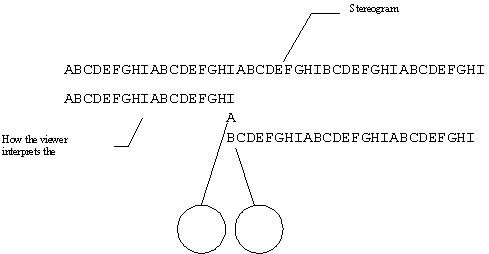
Figure 4-4: 3D interpretation of the missing element

So we now have both a better explanation of why inter-object spacing is so relevant to depth perception, and we have a workable technique for generating depth; if we remove elements from a pattern, we create a step up toward the viewer.

Similarly, if we reintroduce an element to the pattern, a downward step is perceived (the same theory as to why applies; this time the right eye sees an object the left one cannot, so the brain assumes that there is a step down, obscuring the left eye’s view).

We can now construct an elementary stereogram, using the repeated pattern technique, shown below in Figure 4-5. The first two rows are simply the repeated base pattern, so when viewed divergently, these appear below the level of the page. The next 6 rows, however, have had an A removed for 2 repetitions, and then a J introduced to restore the original pattern width of 9 characters. The final two rows are simply the base pattern again. Try viewing this divergently now, and you should see a raised square on the 3^rd to 8^th rows.

· ·

ABCDEFGHIABCDEFGHIABCDEFGHIABCDEFGHIABCDEFGHIABCDEFGHI

ABCDEFGHIABCDEFGHIBCDEFGHIBCDEFGHIJBCDEFGHIJBCDEFGHIJB

ABCDEFGHIABCDEFGHIABCDEFGHIABCDEFGHIABCDEFGHIABCDEFGHI

Figure 4-5: A simple stereogram

We can use this same simple insertion and deletion of pattern elements to produce any complexity of scene; raised objects of any height can be created by removing one or more pattern element and curved surfaces can be created by quantising them to a series of steps toward or away from the user.

However, Figure 4-5 above is lacking in some of the finer points that make a good stereogram; such as an interesting (or random) pattern. It is also rather limited in the scope of depth levels - since to raise a surface we must remove a pattern element, and we are only starting with 9, you can see there is an immediate ceiling on the possible number of depth levels.

4.2 Pattern Substitution

To address the first point, that of the rather dull nature of our first stereogram, we can consider both how we chose our pattern initially, and the independence of the individual rows.

The initial pattern, ABCDEFGHI, was chosen completely arbitrarily. We could equally have chosen STEREOGRAM, 0110101101 or, indeed, any collection of characters or symbols, as it is the repetition of the pattern which is important, not the pattern itself.

Also, since we have determined that the rows within a stereogram are independent, we can choose a new pattern for each line of the image, and as long as all of the patterns chosen are of the same initial length, every line can have a new pattern.

If we create another stereogram, using a base pattern of length 10; 1234567890 (Figure 4-6), we can then choose a substitution pattern for each line to replace this initial pattern. This is shown in Figure 4-7 for a random replacement, using letters of the alphabet.

· ·

123456789012345678901234567890123456789012345678901234567890

12345678901234567890123456789123456789123456789A123456789A12

12345678901234567890123456789123457891234567891A234567891A23

123456789012345678901234567890123478901234567890123456789012

123456789012345678901234567890123456789012345678901234567890

Figure 4-6: Pre-substitution stereogram

· ·

SHYDBUJUKPSHYDBUJUKPSHYDBUJUKPSHYDBUJUKPSHYDBUJUKPSHYDBUJUKP

CZIFBNOKVFCZIFBNOKVFCZIFBNOKVFCZIFBNOKVFCZIFBNOKVFCZIFBNOKVF

GRDMTYAIKXGRDMTYAIKXGRDMTYAIKGRDMTYAIKGRDMTYAIKAGRDMTYAIKAGR

BDFGHJPRKQBDFGHJPRKQBDFGHJPRKBDFGHJPRKBDFGHJPRKABDFGHJPRKABD

GLYNSHERE!GLYNSHERE!GLYNSHEREGLYNSHEREGLYNSHEREAGLYNSHEREAGL

LKJHHBVOBZLKJHHBVOBZLKJHHBVOBLKJHHBVOBLKJHHBVOBALKJHHBVOBALK

THEREPHSTBTHEREPHSTBTHEREPHSTTHEREHSTTHEREPHSTTAHEREPHSTTAHE

POIUYTTREKPOIUYTTREKPOIUYTTREPOIUYTREPOIUYTTREPAOIUYTTREPAOI

UHBTFGSJRQUHBTFGSJRQUHBTFGSJRQUHBTSJRQUHBTFGSJRQUHBTFGSJRQUH

ZJRGDHEKUSZJRGDHEKUSZJRGDHEKUSZJRGEKUSZJRGDHEKUSZJRGDHEKUSZJ

MNBVCCXZSLMNBVCCXZSLMNBVCCXZSLMNBVXZSLMNBVCCXZSLMNBVCCXZSLMN

ABCDEFGHIJABCDEFGHIJABCDEFGHIJABCDEFGHIJABCDEFGHIJABCDEFGHIJ

ZXCVBBNMKLZXCVBBNMKLZXCVBBNMKLZXCVBBNMKLZXCVBBNMKLZXCVBBNMKL

HJKLYUIOPQHJKLYUIOPQHJKLYUIOPQHJKLYUIOPQHJKLYUIOPQHJKLYUIOPQ

Figure 4-7: An (almost) random substitution

4.3 Full Size Stereograms

We now have the basis to generate real stereograms. If you can imagine that, rather than a pattern width of 10 we have a width of 200, and that the individual items of this pattern aren’t letters of the alphabet, but pixels on a computer screen, or dots on a printed page; we can see how a proper stereogram is created.

The process used by the implementation is exactly this. The program first determines a pattern width and output resolution (how many pattern elements the final picture will contain along it’s x and y edges). Then it scans across a depth file (as described in section 0), removing and inserting elements into the pattern as the 3D surface rises and falls. Finally, it replaces this repeated pattern with either random dots, or it performs a colourfield substitution from another graphic file.

The substitution stage of the generation process is the one which most determines how the stereogram will ultimately look. A random selection of colours produces the common RDS variety, more interesting is the colourfield type of stereogram, where each line of the pattern is a line of another, smaller image. This image is then distorted as the pattern elements are inserted and removed, producing a tiled image effect when looked at as a 2D picture, but containing all of the 3D information necessary to view the stereogram illusion.

This process is considered in detail in later chapters; and the algorithms and pseudo code are presented in section 0.

4.4 Advanced Ideas

Now that we have devised a complete technique for generation stereograms, using a repeated pattern, we can discuss some of the issues affecting the quality of output.

Shrink-shift effect

This is a peculiar effect the occurs as the eyes overlay the repeated pattern. If we consider a 10 element pattern ABCDEFGHIJ repeated 4 times (Figure 4-8) viewed divergently, then what we actually see is the pattern repeated 3 times in the centre of the image at the correct depth level, and two ghost images at the edge, caused by one eye seeing the pattern, and the other seeing the blank page.

· ·

ABCDEFGHIJABCDEFGHIJABCDEFGHIJABCDEFGHIJ

Figure 4-8: Shrink-Shift effect

Furthermore, if we consider a raised object in the stereogram, started 20 characters into the image, when viewed divergently, it actually appears displaced to the left, for the same reason; the left-most pattern is lost as only the right eye sees a pattern.

So effectively, the image has been shifted to the left (by one pattern width) and the viewable image area has been reduced (by two pattern widths).

By pre-processing the depth file, we can add a blank area at the far left of the file, thus re-sizing the source image to eliminate the shrinkage, and also providing a new blank area which is lost, rather than the edge of the proper depth image, eliminating the shift.

Anti-Aliasing

If we consider a depth file, containing a raised region (Figure 4-9);

0000000000000000000000000000000000000000000000000

0000000000000000000333333333333333333330000000000

0000000000000000000000000000000000000000000000000

Figure 4-9: simple depth file

When converted to a stereogram, there will be a sharp jump from the background to the object, 3 depth levels above it.

If we anti-alias the depth file (either from within the program, or using an external processor) we can smooth out these discrepancies; and produce a resulting depth file similar to Figure 4-10.

0000000000000000000000000000000000000000000000000

0000000000000000000111111111111111111110000000000

0000000000000000011222222222222222222221100000000

0000000000000001122333333333333333333332211000000

0000000000000000011222222222222222222221100000000

0000000000000000000111111111111111111110000000000

0000000000000000000000000000000000000000000000000

Figure 4-10: An anti-aliased depth file

Now, when the stereogram is created, the image will have a smooth gradient from the background, rather than the harsh (and unnatural) jump that would previously have been created.

Anti-aliasing works better with higher-resolution input files, though, as by necessity it blurs the edges of the objects, reducing their definition in the scene. The larger the object is compared to the area effected by anti-aliasing, the more subtle and effective the result is.

Dual-Direction Stereograms

I also considered an entirely new form of stereogram, or at least one which I haven’t come across in my research, that of hiding two 3D images in one 2D plane.

There are 3 ways this is possible. The first two rely on the fact while the columns in a stereogram are heavily linked for the 3D effect, the rows are independent of each other, so by rotating the image through 90^o, we could conceivable have a second stereogram.

Dual-image linking

This technique would build a linked-list of pixel dependencies across the rows, and then rotate the plane through 90^o and build a second linked-list across (what were) the columns, to encode the second stereogram.

This is a development on the similar pixels technique, rather than colouring the pixels as soon as their neighbour is found, the pairings should be stored in a data-structure.

When this technique is tried, however, due to the complexity of the scenes, and the heavy inter-reliance of pixels, all (or most) of the characters end up linked! This basically means we have found an expensive and time consuming way to fill a page with one colour!

Dual-image interleaving

This idea relies on the random base that stereograms are often built from. The theory is that we can break the final image down into a matrix, and use the 2 sets of pixels (1 and 2 in Figure 4-11) separately for the two stereograms. This removes the added problem of the 2-way pixel dependence of the dual-image linking idea.

1212121212121212121212121212121212121212121212121

2121212121212121212121212121212121212121212121212

1212121212121212121212121212121212121212121212121

2121212121212121212121212121212121212121212121212

1212121212121212121212121212121212121212121212121

2121212121212121212121212121212121212121212121212

1212121212121212121212121212121212121212121212121

2121212121212121212121212121212121212121212121212

1212121212121212121212121212121212121212121212121

2121212121212121212121212121212121212121212121212

1212121212121212121212121212121212121212121212121

Figure 4-11: dual-way stereogram template

The first stereogram uses the pixels marked with a 1 in Figure 4-11 (so the places marked 2 are left blank). The image is then rotated through 90^o, and the second stereogram is formed on the places marked 2, effectively across the columns of the first stereogram. Due to the row-independence; the stereogram should be viewable from either direction without interference.

Alternate pattern width

This again relies on interleaving the stereograms, but this time, rather than rotate the page, the image independence is formed by having the stereograms visible at different depth levels.

Theoretically, using the same grid as designed in Figure 4-11, we should be able to have one stereogram with a width of, say 0.75”, and another at 1.33” (the smaller width must not be an integer divisor of the larger; i.e. 0.75” and 1.5”, as the patterns would interfere); by diverging the eye by different amounts, we should be able to see either stereogram.

Both of the second solutions, although workable, will be very hard to see, and as such haven’t been directly implemented in the software. There is a second program wierdstuff.c planned, which will allow generation of these types of stereogram. The algorithms are pseudo-coded in section 6.4.

4.5 References

For a detailed discussion of the pattern technique, see:

Making Random Dot Stereograms; B Hankinson & A Hermida; QUE, 1994

5. Applications

Before we discuss the implementation, it is useful to take a break from the mathematics and methods of stereo-technology, and see how it is relevant to real-world situations.

Most peoples perception of the role of stereograms (if they have even heard of this phenomenon) is that they are yet another extension of the junk-poster, drop-out culture. Just another gimmick like larva lamps and 3D television programmes.

Many more have never been able to see a stereogram (although they never had my help!) and as such dismiss them as a phenomenon purely based in the fact that if you stare at any weird pattern for long enough, then you’ll think you’ve seen a 3D picture anyway! (Remember those sunny days staring at clouds?!)

We have seen throughout this report, however, that stereograms are more than this, that they are in fact a proper mathematical representation of a 3D scene, carefully disguised to look like they are merely a piece of rejected 1960’s psychedelic art.

There are also more interesting and useful applications for stereograms than the poster/t-shirt/video phenomenon currently gripping high-street poster stores around the country. Stereograms have firm founding in testing, analysing and even fixing problems with individuals depth-perception in medicine and military fields, and stereo technology in general has almost boundless potential.

5.1 Medical Applications

Stereo technology has a number of applications in medicine. The primary topic which was uncovered was, unsurprisingly, that of stereo vision; but this field breaks down into a number of uses for random dot stereograms.

The following information is derived from a number of medical sources, listed in the Bibliography (Section Error! Reference source not found.); direct quotes are referenced.

The use of RDS in medical research can be broken down into a number of categories. There is specific research into factors affecting stereograms, the qualities that make a stereogram viewable, what types of object we can best perceive in a stereogram, and what changes can be made to a stereogram to improve it, or render it non-viewable.

Stereograms are also used in research into how we perceive 3D information; by changing the stimulus and monitoring the physiological effects on the subject, vision in healthy and stereo or motion blind patients can be examined and improved. Forced stimulus of areas of the brain and eyes while looking at a stereogram has also been researched, to see the effect on the subjects ability to see the stereogram.

Neural nets have been proposed and developed using this type of research to try and simulate human vision within a computer system.

There has been a large amount of research on motion perception, using moving random-dot patterns, but this is beyond the scope of the random-dot stereograms examined by this project. There are also a number of issues relating to stereo-perception in general, but again, these are only mentioned briefly.

The references also show that there are a number of ways stereograms themselves can be presented to the viewer. In the case of animal experimentation, because they obviously cannot be trained to view a stereogram (without a great deal of patience, a small miracle and the ability to understand spoken English...) the stereo pairs that can be encoded into one stereogram are actually presented as separate images to the left and right eyes. This is achieved using the various technologies described in chapter 2; such as red/green separation and the strobing of the left and right images onto a computer screen, synchronised with LCD goggles.

Some of the problems of stereograms, such as their lack of any detailed colour information about the object, can be useful in research. Any 3D perception of a stereogram is based purely on spatial information, there are no other depth cues; such as shadows, shading and highlighting of the object. Thus the role of spatial positioning in 3D perception can be examined, isolated from other possible sources of depth information.

Due to the large quantity of references on the subject of stereo-technology, I have attempted to cover a wide range of subjects fairly briefly, rather than any specific field in detail; especially due to the non-medical nature of the project. However, I feel the real-world applications of this project are as (if not more) important than the mechanics of stereogram generation.

Stereo Research

If we first examine the issues directly relating to stereogram technology, we can see that there has been some interesting research on the subject.

In Vision Research[ii], the effect of adding random noise to stereograms is examined. The individual dots of the stereogram were corrupted, and the study found that ‘When the stimulus was a random dot stereogram in which perturbations of disparity were applied independently to each dot, most of the dots had very different disparities from their neighbours and efficiency was found to fall as the level of disparity noise was increased’. The study goes on to conclude that this is due to the decreasing ability of the eyes to match the stereo-paired dots as the distortion is increased. They proved this by distorting the image as a whole, while keeping the relationship constant between the stereo-pairs.

As we have continually seen while discussing the theory of stereograms, this inter-pair linking is the most important aspect of simulated depth, and this study supports that hypothesis.

In a similar study, the effect of blurring of vision on stereogram viewing was tested. A strict mathematical relationship between blurring and stereogram perception was found (Optometrist Visual Science[iii]). This knowledge provided, they concluded, ‘a rationale for the use of random element stereograms for the detection of refractive amblyopia and ametropia in the vision screening of children’

The users ability to accurately distinguish objects in a stereogram is related to the dot-distribution. In a stereogram with 50:50 black:white, the viewer can most accurately pinpoint the corners of a shape, but as the image is biased towards either black or white, the definition is lost[iv].

This fact can be visually verified by generating two stereograms using my software, one with a 50/50 ratio, and another with, say 15% white dots. It is clear when the white-biased stereogram is viewed that it is not as clearly defined. This can also be related to colourfield stereograms: a base pattern with large plain areas is not a good choice, as resolution will be lost in these regions. An erratic pattern with lots of colour and shape changes works far better, as the calculated distortions are more likely to be visible in the repeated pattern.

A study into shape-recognition using stereograms in Perceptual Psychophysics[v] revealed that some 3D objects are easier to recognise than others. While elliptic (and, of course, simpler shapes) were easy to recognise, hyperboloid surfaces are slightly harder to distinguish. The extent of the curve, or the size of the object had little or no effect on it’s recognisability. This helps to explain why some regions of a stereogram are harder to see than others; the brain is more likely to accept the 3D information for a simple object, than the complex information required to encode a more intricate object.

At various points in this report I have implied that the eyes and brain can be trained to see stereograms; and this would need seem to be true by the fact that they do get easier to see, the more you look at. In Perception[vi], a study revealed that ‘evidence was obtained that suggests that observers can learn, to a certain degree, monocular random-dot patterns and that this learning facilitates the depth percept’. Practice really does make perfect with regards to stereo-vision.

As mentioned in chapter 3.5, stereogram technology is hampered by the time taken to generate the stereogram, limiting it’s real-time applications. In mid-1994, Gonzalez & Krause[vii] devised a system which could solve this problem, based around a cheap Amiga 500 computer, slaved to another desktop.

Research into stereo vision has even led to neural-net development, leading to a system capable of developing the ability to see 3D surfaces within a random-dot stereogram. (Nature[viii]).

Use of RDS in examination of depth perception

Experiments into the effect of stimulus on stereo vision range from the sublime to the macabre. In the Journal of Neurology[ix] an experiment in which a magnetic field was induced by the head of a subject while they were viewing a stereogram, through red/green goggles is described. The stimulus did indeed cause temporary loss of stereo vision; ‘Repetitive magnetic stimulation easily and painlessly produced a reversible disturbance in global stereopsis’. Their experiments confirmed the hypothesis about the location of one of the brains stereo-perception centres.

The advent of stereogram technology has allowed scientists to examine sight at a lower level that was previously possible. In Perception[x], the authors aimed to examine the process of depth perception using purely spatial information. ‘Exploration of the human visual processing system at this level is, however, extremely difficult, but can be facilitated by the use of stroboscopic presentation of sequences of random-dot stereograms’.

This type of research, using RDS and other stereo technology has revealed a great deal about human (and animal) perception of depth. Issues such as visual resolution, ability to detect motion, use of visual hints in depth perception (as previously mentioned) have all benefited from research using stereograms.

Random-dot test are also widely used to monitor the development of vision in children and the visually impaired, and a number of references are included on these tests; due to the technical nature of the articles, I have decided not to discuss them here. However, one report finds a Random-dot E test to be ‘one of the most effective in examining childhood sight deficiencies’[xi].

Stereograms have also been used in a number of tests on animals; monitoring physiological responses to random-dot stimuli. For example, in Vision Research[xii], a squirrel monkey was (successfully) tested for stereo-vision.

A comparative study of 3D stereo technologies discovered that ones using polarised light were no more effective or valid than those (such as random-dot) which were viewed normally, again justifying the use of stereograms in medicine[xiii].

Motion perception

Various references to the use of stereo-kinetic motion tests, including random-dot techniques are included in the bibliography.

Stereo Technology in General

In medicine, general stereo-technology has a number of applications. Almost any kind of imaging system can be enhanced by adding a second lens, and combining the sources into a stereo image. For example, techniques have already been devised for keyhole surgery cameras, and laproscopes & endoscopes (see Endoscopic Surgery Allied Technology[xiv] and Surgical Endoscopy[xv])

There has also been some worrying research into the widely used VR headsets, both in commercial and industrial applications. In a survey in 1993[xvi], the authors discovered that the average stereo separation that these devices supply to the user, together with the erratic speed of the output caused eyestrain and other trauma to a number of users.

5.2 Military Applications

By the very nature of the military, I had difficulty finding military references to stereograms.

There was, however, one source detailing the problems of testing pilots using the Verhoeff Stereopter. The study (by S Beckerman & D Lee[xvii]) examines the case of an officer who failed a stereo-vision test performed with the Stereopter. They re-tested him using randot tests, based on the same basic theory as our random-dot stereograms, and discovered that it was the procedure that was at fault, rather than the subject’s stereo-vision.

This use of random-dot technology has therefore helped to highlight a problem with the military’s testing procedure, and indeed the author’s concluded that ‘Although this instrument is not popular among vision care practitioners, it is being utilised by various organisations’. In using the randot test to verify the Verhoeff results, they clearly felt that RDS technology was a good test of stereo-vision.

5.3 Industrial Applications

As discussed in section 0, chemical companies commonly use the LCD goggles based 3D imaging systems, to study, adapt and develop complex organic molecules.

6. Software Design

The implementation for this project is quite a low-scale one. The real challenge of the project was on finding the best way to generate stereograms of various kinds, while allowing a large degree of flexibility in the output parameters of the file.

A number of generation techniques were considered; indeed two different ways were implemented in the prototype, but due to it’s simplicity and versatility, the Pattern Substitution Technique described in chapter 0.

6.1 Data Flow Diagrams

The stereogram generator takes input of a depth file and the parameters to determine the style of the stereogram (pattern width, dpi, resolution etc.). These parameters can either be specified by the user, or the program will use it’s defaults.

If a colourfield stereogram is to be generated, the program also needs to input that file (shown by the dashed line in the overview diagram, Figure 6-1)

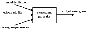
Figure 6-1: Overview

We can break down the data-flow within the main program further;

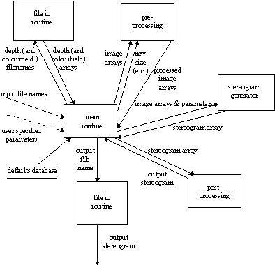
Figure 6-2: expanded data-flow diagram

6.2 Program Structure

The program itself is broken down into a number of sub-procedures; as illustrated by the data-flow diagram (Figure 6-2). These are:

· main.c
Deals with the command-line interface, setting the parameters to those chosen by the user or to the internal defaults. It also controls the flow of data through the other routines.

· stereo.h
contains default parameters, and configuration information for the program

· fileio.c
reads the actual images (depth and colourfield) and writes an output file containing the stereogram. All of these files are in the PPM Portable Pixmap format

· preprocess.c
Handles file scaling (to get the input files to the correct resolution); depth scaling (as mentioned before, a stereogram’s depth file should be processed to remove extreme changes, as this will create an impossible to view image) and any other changes that must be made to the file before it is converted into a stereogram. This routine also performs shrink-shift compensation, also mentioned earlier. It could anti-alias the input file to remove harsh edges from the finished 3D illusion

· postprocess.c
Performs finishing operations on the stereogram to be output; such as smoothing, colour-reduction; and processing to produce the multi-stereogram output files discussed earlier.

There are other .h header files, containing configuration data, but these are purely internal to the program.

6.3 Algorithm Pseudo Code

We can now detail the pseudo code used in both the original prototype, and in the final program.

Both algorithms work from a 256 level depth file, with value 0 being the furthest from the viewer, and value 256 being the nearest.

Algorithm 1 - Similar Pixels Technique

This is the simplest algorithm for generating RDS stereograms. It’s basic operation was discussed in chapter 0, but here we attempt to explain it more formally.

This first section initially fills the image file with a random pattern.

For each line of the depth file {

For each pixel n in turn {

pixel n in imageFile = genRandVal

}

The second section then takes this random file and according to the corresponding depth values in the depth file, ensures that linked pixels (needed to create the 3D illusion) are the same colour (0 or 1).

The depthFactor variable is used to scale the number of depth levels from 256 (in the depth file) to the number on screen. For example, a 16 level image would need a depthFactor of 16.

For each line of the depth file {

For each pixel n in turn {

read depthVal = the depth value of pixel n

set linkedPixel = [n + (256 - depthVal) / depthFactor]

If [linkedPixel < lineWidth] {

pixel linkedPixel in imageFile = pixel n in imageFile

}

This algorithm could be modified to generate colourfield stereograms, by replacing genRandVal with a more sophisticated routine to distort an input tileable pattern. However, the variable depthFactor is an unsatisfactory way to vary the number of levels in the final image.

As we have already seen, though, the pattern substitution method is far more suited to generating colourfield (and RDS) images, so we will detail this algorithm now:

Algorithm 2 - Pattern Deletion and Insertion

This is the more complex algorithm (using pattern element deletion and insertion) allowing both RDS and colourfield stereograms using an intermediate pattern file. This is the technique used in the completed software.

The variable depthLevels defines the number of levels to be present in the final image, and is determined by the program from the input parameters and default values.

Main Loop

This algorithm takes the depth file and creates the intermediate pattern file.

For each line of the depth file {

maxNumber = depthLevels

Initialise the pattern using depthLevels

For each pixel n in turn {

difference = depthValue of pixel n - depthValue pixel n-1

If difference > 0 { /* pixel is nearer than the previous one */

delete [difference] elements from the pattern

Else If difference < 0 { /* pixel further away */

insert [difference] elements into the pattern

}

} /* else pixel is at the same level */

pixel n in patternFile = pattern[nextElement]

increment nextElement mod patternWidth

}

Pattern Deletion algorithm

This algorithm removes ‘difference’ elements from the current position (nextElement) in the pattern file, thus varying the pixel separation and creating the depth information.

tempPattern = pattern

set newPatternWidth = patternWidth - difference

set newNextElement = nextElement + difference MOD patternWidth

For each element n in pattern {

pattern[n] = tempPattern[newNextElement]

increment newNextElement MOD patternWidth

}

patternWidth = newPatternWidth

nextElement = 0

Pattern Insertion algorithms

This algorithm inserts ‘difference’ elements into the pattern. This can be done in a number of ways, each suits a different type of stereogram better.

Technique 1 - best for RDS as it randomises the elements even more.

This simply adds ‘difference’ new (never before used) elements to the pattern.

This technique needs a new variable; maxNumber. This is set when the pattern is created to ‘depthLevels’ and is used to create new, never before used pattern elements.

tempPattern = pattern

set newPatternWidth = patternWidth + difference

next = 0

count = 0

Do until count = difference{

pattern[next] = maxNumber + count

increment count

increment next

}

For each remaining element n in pattern {

pattern[n] = tempPattern[nextElement]

increment nextElement MOD patternWidth

}

patternWidth = newPatternWidth

maxNumber = maxNumber + difference

nextElement = 0

Techniques 2 - best for Colourfields as it reduces base-image distortion.

This technique re-inserts old, deleted pattern elements, into the pattern.

Although it performs a more complex operation, this algorithm is shorter, as it doesn’t need to keep referencing the current pattern; as it is always trying to re-create as much of the original pattern as possible. It achieves this by setting the value ‘index’ to ‘difference’ elements back in the original pattern (modulo pattern width) and then simply writing out the number of elements mow required in the pattern.

index = (pattern[nextElement] - difference) MOD depthLevels

patternWidth = paternWidth + difference

For each element n of pattern {

pattern[n] = index

increment index MOD depthLevels

}

nextElement = 0

Substitution Algorithms

The next algorithms take the pattern file and perform pattern substitutions on it, taking the non-random pattern file and replacing it with an RDS or colourfield stereogram. This substitution ideally needs to take place across each line, saving memory and reducing the number of variables needed; so these algorithms need to be integrated into the end of the main loop.

RDS Substitution

This takes the pattern file and simply replaces each number within it with a random value. It needs a new array substVals of length ‘maxNumber’ as this variable indicates the greatest value used in the pattern. (This substitution technique therefore works well with the RDS pattern insertion algorithm described earlier).

For each line of the Pattern File {

For each element n of the substVals array {

substVals[n] = genRandomVal

}

For each pixel m of the image file {

imageFile[m] = substVals[(patternFileLine[m])]

}

genRandomVal is a separate algorithm which will produce a random value; be it monochrome or colour. This algorithm will be able to bias the selection to vary pixel density, colour variance etc. to create a ‘nicer’ random image.

Colourfield Stereogram Substitution

This takes the pattern file and a smaller, base-image from which it derives a substVals array. If we have variables Line, the current line of depth file; and fieldLines, the number of lines in the colourfield tile image; the substVals array is taken to be the (line MOD fieldLines) line of the colourfield.

For each line ‘line’ of the Pattern File {

For each pixel m of the image file {

imageFile[m] = colourfield[(line MOD fieldLines)*depthLevels +

(patternFileLine[m]))]

}

6.4 Weird Stuff Algorithms

These algorithms are designed to be used in conjunction with stereograms generated by the main program.

2-Way

This algorithm should be run on two stereograms, generated at either half the required pattern width, of half the output dpi. The stereograms should be square, and the final stereogram will also be square, but twice the size of the original sources (i.e. two 400x400 stereograms, pattern width 0.5” will produce an 800x800 2-way stereogram, pattern width 1”)

This operates on the two original stereograms, stereo1 and stereo2, and produces stereogram.

/* first stereogram */

For ( row=0 ; row < xres ; row ++ )

For ( column=0 ; column < columns ; column ++ )

if row is even

stereogram(row*2,column*2) = stereo1(row/2, column/2)

else

stereogram(row*2,column*2+1) = stereo1(row/2, column/2)

/* second stereogram */

For ( row=0 ; row < xres ; row ++ )

For ( column=0 ; column < columns ; column ++ )

if row is even

stereogram(column*2,row*2) = stereo1(row/2, column/2)

else

stereogram(column*2,row*2+1) = stereo1(row/2, column/2)

This should interleave the stereograms effectively, and because the resolution has effectively been halved, the pattern width will now be doubled back to the correct size.

Dual Level

This again requires some work on the users part, but would ideally be a fully integrated function. Two stereograms of the same resolution should be generated, but with different and non divisible pattern widths (i.e. 1” and 1.75”).

These stereograms would again be interleaved, but this time, they would both be visible in the same orientation of the stereogram, but the user would have to diverge their eyes by different amounts to see each one.

However, by experimenting with this technique, I have discovered that it cannot work; the eye, when focused through the 2D plane simply manages to see both stereograms at once, with a large amount of interference.

If we consider again the theory of stereograms, it is clear that this will happen; the eye just interprets the second stereogram as a distortion of the pattern of the first, and fails to distinguish between the two.

7. Software Implementation & Evolution

7.1 Prototype Design

The prototype was designed purely to test the validity of the Similar Pixels and Repeated Pattern Technique algorithms discussed in section 0. It uses internal functions to generate a depth map, and used a simple 1-bit PPM file read/write procedure to produce an RDS output file.

The software and stereogram configuration had to be performed by editing internal variables.

In it’s final versions, the prototype also implemented colourfield stereograms, from a 1-bit PPM file, and the original code implementing the Similar Pixels Technique was removed, now rendered redundant by the newer, more versatile Repeated Pattern ones.

Problems Encountered

The prototyping stage revealed a number of problems with stereogram generation.

The first problem highlighted was that discussed in section 0; the problem of the maximum number of depth levels that could be used. It soon became clear when attempting to view the output stereogram that some tailoring of the range of values in the depth file (at this time internally generated) was required before the stereogram could be generated. The greatest depth in the input file had to be considerably lower than the theoretical maximum number of levels, to enable the algorithms to complete without error, and to produce a viewable stereogram.

The second point was that of handling the large arrays required to hold a screen or printer resolution image. Even at this stage, dealing purely with monochrome images, it was clear that there would need to be a compromise between speed and efficiency. Heavy use of C’s pointers has been made to try and reduce the amount of memory used in both the prototype and final versions.

The more advanced pattern-insertion algorithm, listed in section 0 was found to be flawed; causing an undesirable ghosting effect due to interference with the previous patterns. The slightly simpler colourfield insertion algorithm has therefore been used in the implementation.

It also became clear that the program would need to be intelligent when dealing with it’s input files. When generating a colourfield stereogram, for example, for the best results, the colourfield tileable pattern needs to be of the same x-resolution as the pattern width, if it is to tessellate properly. Users cannot always be relied on to provide such convenient input, and it was decided that the software would have to deal with as many of these type of input requirements as possible.

7.2 Command Line Interface (CLI) design

The user had to be able to specify exactly what they wanted of the programme, but without having to specify every parameter effecting the output file. For instance, they may wish to define the output resolution of the image, but not really worry about the initial pattern width. To this end, there are a number of program defaults (specified in stereo.h) that the software will use unless the user overrides them using input parameters.

There is a full discussion of the user interface in the user manual, section 9.3.

7.3 Full Implementation

The final implementation required a complete re-write of the program, as the internal representation of the image was incompatible with the PPM libraries chosen to aid graphic file input and output.

The PPM libraries are provided with the UNIX OS, and as such are heavily documented, so they will not be discussed in this report.

The command line interface was implemented at this stage, and the original component functions of the prototype were grouped and broken down into separate source files. The necessary alterations were made to the existing functions, to deal with the new graphic file representation; and a number of new routines were added:

· Image resizing

To deal with both the output resolution, and scaling of the input colourfield file to make it suitable for the calculated pattern width

· Shrink-shift

To deal with the shrink-shift effect discussed in section 0 It was decided that if the user specified an output resolution, this would be the size of the image after the shrink shift algorithm had been used, else the output file would be slightly wider than the input depth file, having applied shrink shift to it. (e.g. if the depth file is 400x400; 100 levels, user specifies 800x800 output: depth file is initially resized to 700x800, then shrink-shifted to 800x800. If the user hadn’t specified an output size, the 400x400 file would be shrink-shifted, producing a 500x400 output; retaining the input file’s aspect ratio and original size when viewed stereoscopically).

· Depth Scaling

The depth file is taken and processed such that the greatest depth level is equal to half the pattern width. While this reduction is on the cautious side, it is far more likely to produce a viewable stereogram.

· Dot Routine

A simple procedure to add the two dots to the top of the image, as a viewing guide for the user (as discussed in section 0).

File Formats

The software requires up to two input files; the depth map and the colourfield. It outputs the stereogram in a 24-bit PPM file.

· Depth Map

This file should be a 24-bit PPM file. The program judges the depth of the object by the red component of it’s 24-bit value; allowing for 256 possible depth levels. The 24-bit format was chosen both as it is a common file-format and because of the future expansion that could be made by using the blue and green components to specify the 3D depth position even more accurately.

The easiest way to visualise a depth file is to start with a black canvas, and draw in various shades of grey on it, starting with the darkest colours, forming distant objects, and ending with white; forming the nearest objects. Since the colours are all grey, there will be the correct linearity of red-colouration in the file, creating the correct depth levels.

· Colourfield File

This can be any P?M filetype, although a grey-scale PGM or non dithered colour PPM should be used, as the program is likely to resize the input file. It uses a linear re-scaling algorithm, which would not work well when resizing a dithered image.

· Output File

The program outputs a 24-bit PPM file, which can then be converting to any other file-format (such as TIFF or Post Script) using the PBMPLUS library of tools (e.g. ppmtotiff or pnmtops) or displayed and converted using the XV software. There are many other file-converters and viewers available that will deal with PPM files on UNIX systems, and a few (such as Paint Shop Pro, version 3 or above) on MSDOS and other systems.

For the best results, 24-bit, un-dithered input files should be used.

8. Conclusions and Future Work

8.1 Project Achievements

As intended, the project has examined many aspects of 3D stereo technology; including stereograms in some detail.

Various techniques for stereogram generation were researched, and both the linked-pixel and repeated pattern techniques have been implemented.

The software is capable of producing both the Random Dot and Colourfield types of stereogram. It also attempts to overcome some of the problems associated with stereogram generation, such as the shrink-shift effect, and tailoring of the input depth file.

There are many ways the user can alter the output parameters of the stereogram; from the type of device it will be displayed on to the pattern width of the stereogram itself.

8.2 Problems and Possible Developments

The project still has scope for development.

A full graphical interface would be preferable to the command line interface currently implemented. This could include a thumbnail of the depth image and of the colourfield file, as well as a representation of the final output stereogram.

The stereogram generator itself could be improved to reduce colourfield image distortion. Currently, as elements are deleted from the pattern, they are lost forever. When an element is inserted, it is copied from elsewhere in the current pattern. It would be preferable if old elements could be re-used, but the algorithm developed to do this was flawed (as mentioned earlier).

Generation of a stereogram animation is possible with this software, but the animation would have to be developed elsewhere and converted one frame at a time.

A slight lack of artistic ability and a time constraint (plus some teething trouble with printing the laser-resolution output files) has led to a distinct lack of stereograms in this report. Hopefully, there will be full complement available for the demonstration, and to be slotted into Appendix 10.3

Further work needs to be done on the ideas for multi-direction and multi-stereogram images. This are only implemented in an elementary form, and should be presented in a fully enclosed environment.

9. Software Manual

9.1 Using GJG’s Stereogram Generator

This piece of software has been designed to produce both types of stereogram discussed in this report; Random Dot Stereograms (RDS) and Colourfield (or Tiled Pattern) stereograms. It does this by taking an input depth file.

This depth file should contain the objects you wish to be present in 3D in the final stereogram, coloured such that black is the farthest plane in the image, and white is the nearest. The greys in-between form the various intermediate depths.

The software can either produce a seemingly random pattern of dots, or it can also take a smaller, preferably tileable image as input, and distort this file across the width of the stereogram, thus encoding the 3D information.

9.2 User Options

There are a number of ways to tailor the output of the stereogram, ranging from the type of the stereogram to the mathematical parameters used to generate it.

Both the pattern width (which, for divergent stereograms should be between approximately 0.66” and 2”) and the output device dpi (e.g. screen is around 100 dpi, and a laser printer is usually 300 dpi). These parameters are multiplied to give the number of possible depth levels in the final image.

Either type of stereogram; random-dot or colourfield, can be selected as the output type.

9.3 Command Line Interface

The stereogram generator can be run from the command-line, the format is as follows:

stereo [-r | -c colourfield] -d depthfile -o outputfile

{-x xres -y yres -s -l} {-p white_percent}

{-i dpi -w width}

{-m}

-r specifies an RDS output

-c specifies both colourfield output, and the base image to be used.

-m specifies that the middle-out technique should be used, to reduce distortion of the tiled pattern

-x and -y specify the resolution of the output file

-i sets the output device dpi (in pixels per inch)

-s sets the above options automatically to generate a screen resolution (1152x900, 100 dpi)

-l sets the above for laser printer resolution (3300x2400, 300 dpi)

-w sets the pattern width (in inches)

-p sets the percentage of white dots to be used in RDS output

You must specify at least input (depth file) and output filenames (-d name and -o name), the software will use it’s default values for the other options unless they are specifically stated.

The command line options are processed in list order - contradictory options (such as specifying the filename twice) will result in the last instance on the command line being taken as the correct one.

For example, if you wish to generate an RDS stereogram from a depth file called depth.ppm to an output output.ppm;

stereo -d depth.ppm -o output.ppm

If you want to generate a colourfield from the same depth file, and colourfield file cf.ppm, with final resolution 1024x768;

stereo -d depth.ppm -o output.ppm -c cf.ppm -x 1024 -y 768

You can, of course, specify any of the other options, such as to change the pattern width to 1.5” (-w 1.5) or to change the dpi to 128 (-i 128).

10. Appendices

10.1 Code

This section contains the code as it stood in Version 1.90, 16/06/95. There are some functions still to be debugged and implemented before the demonstration.

main.c

#include <stdio.h>

#include <stdlib.h>

#include "stereo.h"

#include "fileio.c"

#include "algs.c"

#include "preprocess.c"

#include "postprocess.c"

void

main( int argc, char *argv[] )

{

pixel **depthfile, **outputfile, **cfield;

extern int xres, yres, dpi, percent, stereo, levels;

int c, cfx, cfy, dpx, dpy, tmp;

int scale=FALSE;

extern float width;

float factor;

pixval cfmax, dpmax, opmax;

char *depth, *output, *colour;

stereo = RDS;

xres=yres=-1;

factor=0.0;

depth=output=colour=NULL;

/* defaults */

percent=PERCENT;

dpi=DPI;

width=WIDTH;

while (argc > 0)

if (--argc > 0 && (*++argv)[0] == '-')

{

c = *++argv[0];

switch (c)

{

case 'r':

stereo = RDS;

break;

case 'x':

xres = atoi(*(argv+1));

scale = TRUE;

break;

case 'y':

yres = atoi(*(argv+1));

scale = TRUE;

break;

case 'i':

dpi = atoi(*(argv+1));

break;

case 'w':

width = atof(*(argv+1));

break;

case 'p':

percent = atoi(*(argv+1));

break;

case 'd':

depth = *(argv+1);

break;

case 'o':

output = *(argv+1);

break;

case 'c':

colour = *(argv+1);

stereo = CFIELD;

break;

case 'l':

dpi = 300;

xres = 3300;

yres = 2400;

scale = 1;

break;

case 's':

dpi = 100;

xres = 1152;

yres = 900;

scale = 1;

break;

case 'a':

stereo = REPLACE;

break;

case 'f':

factor = atof(*(argv+1));

scale = 1;

break;

default:

fprintf(stderr, "Invalid option '%s'\nQuitting.\n", *argv);

exit(0);

break;

}

levels = width*dpi;

if (!depth)

{

printf("Must specify '-d [depth file name]'\n");

exit(1);

}

if (!output)

{

printf("Must specify '-o [output file name]'\n");

exit(1);

}

printf("Depthfile: ");

depthfile = read_image(depth, &dpx, &dpy, &dpmax);

if (xres<1) xres = dpx;

if (yres<1) yres = dpy;

if (factor) {xres *= factor; yres *= factor;}

printf("xres=%d, yres=%d, dpi=%d, width=%f, levels=%d\n", xres, yres, dpi, width, levels);

printf("depth=%s, colour=%s, output=%s\n", depth, colour, output);

if (stereo)

{

printf("Colourfield: ");

cfield = read_image(colour, &cfx, &cfy, &cfmax);

tmp = (int) (cfy * (float) levels/cfx);

cfield = scale_image (cfield, cfx, cfy, levels, tmp);

cfx = levels;

cfy = tmp;

}

if (xres<1) xres = dpx;

if (yres<1) yres = dpy;

if (scale)

{

xres = xres-levels;

printf("Depthfile: ");

outputfile = scale_image(depthfile, dpx, dpy, xres, yres);

}

else

outputfile = depthfile;

opmax = dpmax;

if (STEREOG)

{

printf("Depthfile: ");

scale_depth(outputfile, xres, yres, &dpmax);

outputfile = shrink_shift(outputfile, &xres, yres);

stereogram(outputfile, xres, yres, cfield, cfx, cfy);

add_dots(outputfile, xres, yres);

}

printf("Output: ");

write_image(output, outputfile, xres, yres, opmax);

}

stereo.h

/* truths */

#define FALSE 0 /* truths */

#define TRUE 1

/* constant identifiers */

#define RDS 0 /* non-zero causes colourfield read */

#define CFIELD 200

#define REPLACE 300

/* programme parameters */

#define RAWPPM 0 /* raw or compressed ppm output */

#define STEREOG TRUE /* make stereogram? */

#define LPC 50 /* percent of levels in depth file to use */

/* defaults */

#define PERCENT 50

#define DPI 128

#define WIDTH 1.5

int xres, yres, dpi, percent, stereo, levels;

float width;

algs.h

void init_pattern (int *pattern, int *pattern_width, int *patternP, int *max_number);

void delete (int difference, int *pattern_width, int *patternP, int *pattern);

void insert (int difference, int *pattern_width, int *patternP, int *pattern, int *max_number);

void substitute (pixel **image, int y, pixel **cfield, int cfx, int cfy, int max_number);

algs.c

#include <stdio.h>

#include <stdlib.h>

#include <ppm.h>

#include "stereo.h"

#include "algs.h"

void

stereogram(image, xres, yres, cfield, cfx, cfy)

pixel **image, **cfield;

int xres, yres, cfx, cfy;

{

int x, y, pattern_width, patternP, max_number;

int current, previous, difference;

int pattern[levels];

printf("Converting to Stereogram\n");

srand(time(NULL));

for ( y=0 ; y<yres ; y++ )

{

current=0;

init_pattern (pattern, &pattern_width, &patternP, &max_number);

for ( x=0 ; x<xres ; x++)

{

previous = current;

current = PPM_GETR( image[y][x] );

difference = current - previous;

if (difference>0)

delete(difference, &pattern_width, &patternP, pattern);

else if (difference<0)

insert(-difference, &pattern_width, &patternP, pattern, &max_number);

patternP = (patternP + 1) % pattern_width;

PPM_ASSIGN( image[y][x] , (pattern[patternP]), 0, 0);

}

substitute( image, y, cfield, cfx, cfy, max_number);

fprintf(stderr,".");

}

printf("\n");

}

void

init_pattern (pattern, pattern_width, patternP, max_number)

int *pattern, *pattern_width, *patternP, *max_number;

{

int i;

*pattern_width = levels;

*patternP = 0;

*max_number = levels;

for ( i=0 ; i<levels ; i++ )

pattern[i] = i;

}

void

delete (difference, pattern_width, patternP, pattern)

int difference, *pattern_width, *patternP, *pattern;

{

int newPatternWidth, newPatternPtr, i;

int tempPattern[*pattern_width];

for (i=0; i<*pattern_width; ++i)

tempPattern[i] = pattern[i];

newPatternWidth = *pattern_width - difference;

newPatternPtr = (*patternP+ difference) % *pattern_width;

for ( i=0 ; i<newPatternWidth ; ++i)

pattern[i] = tempPattern[newPatternPtr++ % *pattern_width];

*pattern_width = newPatternWidth;

*patternP = 0;

}

void insert (difference, pattern_width, patternP, pattern, max_number)

int difference, *pattern_width, *patternP, *pattern, *max_number;

{

int temp_pattern[levels];

int i, newPatternP, newPatternWidth, count=0, index;

switch (stereo)

{

case RDS:

newPatternWidth = *pattern_width + difference;

for (i=0; i<newPatternWidth; ++i)

temp_pattern[i] = pattern[i];

do {

pattern[count] = *max_number + count++;

} while (count != difference);

for (i = difference; i < newPatternWidth; i++)

{

pattern[count++] = temp_pattern[*patternP % *pattern_width];

*patternP = (*patternP + 1) % *pattern_width;

}

*pattern_width = newPatternWidth;

*max_number = *max_number + difference;

*patternP = 0;

break;

case CFIELD:

for ( i=0 ; i<*pattern_width ; i++)

temp_pattern[i] = pattern[i];

*patternP = (*patternP - difference) % *pattern_width;

newPatternP = 0;

newPatternWidth = *pattern_width + difference;

for (i=0; i<newPatternWidth; i++)

{

pattern[i] = temp_pattern[*patternP];

*patternP = (*patternP + 1) % *pattern_width;

}

*patternP = 0;

*pattern_width = newPatternWidth;

break;

case REPLACE:

index = ( (pattern[(*patternP) % *pattern_width])

- difference + levels) % levels;

*pattern_width = *pattern_width + difference;

for ( i=0 ; i<*pattern_width ; i++)

pattern[i] = index++ % levels;

*patternP = 0;

break;

}

void

substitute (image, y, cfield, cfx, cfy, max_number)

pixel **cfield, **image;

int y, cfx, cfy, max_number;

{

int subst[max_number];

int x, i, random, boundary, val, index;

pixval r,g,b;

switch (stereo)

{

case RDS:

boundary = (int) RAND_MAX * ((float) percent / 100);

for ( i=0 ; i<max_number ; i++ )

{

random = rand();

(random < boundary) ? (subst[i] = 1) : (subst[i] = 0);

}

for ( x=0 ; x<xres ; x++ )

{

val = 255 * subst[PPM_GETR(image[y][x])];

PPM_ASSIGN ( image[y][x], val, val, val );

}

break;

case CFIELD: case REPLACE:

for (x = 0; x < xres; x++)

{

index = PPM_GETR(image[y][x]);

r = PPM_GETR ( cfield[y % cfy][index] );

g = PPM_GETG ( cfield[y % cfy][index] );

b = PPM_GETB ( cfield[y % cfy][index] );

PPM_ASSIGN ( image[y][x], r, g, b);

}

preprocess.c

#include <stdio.h>

#include <ppm.h>

#include <pbmplus.h>

#include "stereo.h"

void

red(image, cols, rows)

pixel **image;

int cols, rows;

{

int x,y;

pixval val;

printf("Greyscaling (for red depth)\n");

for (y=0; y<rows; y++)

{

for (x=0; x<cols; x++)

{

val = PPM_GETR(image[y][x]);

PPM_ASSIGN( image[y][x], val, val, val);

}

pixel **

scale_image(image, cols, rows, newx, newy)

pixel **image;

int cols, rows, newx, newy;

{

pixel **newimage;

int x, y;

float xstep, ystep, i=0, j=0;

printf("Scaling image to %dx%d\n", newx, newy);

newimage = ppm_allocarray( newx, newy );

xstep = (float) cols/newx;

ystep = (float) rows/newy;

for ( y=0 ; y<newy ; y++ )

{

for ( x=0 ; x<newx ; x++ )

{

newimage[y][x] = image[(int)j][(int)i];

i += xstep;

}

j += ystep;

i=0;

}

ppm_freearray(image, rows);

return newimage;

}

void

scale_depth(image, cols, rows, maxval)

pixel **image;

int cols, rows;

pixval *maxval;

{

int x,y;

pixval newval=LPC;

printf("Depth scaling %d%%...\n", newval);

for ( y=0 ; y<rows ; y++ )

for ( x=0 ; x<cols ; x++ )

{

PPM_DEPTH( image[y][x], image[y][x], *maxval, newval);

}

pixel**

shrink_shift(image, cols, rows)

pixel **image;

int *cols, rows;

{

pixel **newimage;

int x, y;

newimage = ppm_allocarray( (*cols+levels), rows);

for ( y=0 ; y<rows ; y++ )

{

for (x=0 ; x<levels ; x++)

PPM_ASSIGN(newimage[y][x], 0, 0, 0);

for ( x=0 ; x<*cols ; x++ )

newimage[y][x+levels] = image[y][x];

}

*cols += levels;

return newimage;

}

postprocess.c

#include <stdio.h>

#include <ppm.h>

#include <pbmplus.h>

#include "stereo.h"

void

add_dots(image, xres, yres)

pixel **image;

int yres, xres;

{

int middle, x, y, dot1, dot2;

printf("Adding dots..\n");

middle=xres/2;

dot1=middle-levels/2-xres/50;

dot2=dot1 + levels;

for ( y=yres/100 ; y<yres/100 + xres/75 ; y++ )

{

for ( x=dot1 ; x<dot1+xres/75 ; x++)

PPM_ASSIGN( image[y][x], 0, 0, 0);

for ( x=dot2 ; x<dot2+xres/75 ; x++)

PPM_ASSIGN( image[y][x], 0, 0, 0);

}

fileio.c

#include <stdio.h>

#include <ppm.h>

#include "stereo.h"

pixel**

read_image(fn, colsP, rowsP, maxvalP)

char *fn;

int *colsP, *rowsP;

pixval *maxvalP;

{

FILE *fp;

pixel **image;

printf("Reading %s\n", fn);

if ((fp = fopen(fn, "r")) == NULL)

{

fprintf(stderr, "Can't open file %s\n", fn);

exit(1);

}

else

{

image = ppm_readppm(fp, colsP, rowsP, maxvalP);

fclose(fp);

}

return image;

}

void

write_image(fn, image, cols, rows, maxval)

char *fn;

pixel **image;

int cols, rows;

pixval maxval;

{

FILE *fp;

printf("Writing file %s\n", fn);

if ((fp = fopen(fn, "w")) == NULL)

{

fprintf(stderr, "Can't open file %s\n", fn);

exit(1);

}

else

{

ppm_writeppm(fp, image, cols, rows, maxval, RAWPPM);

fclose(fp);

}

10.2 Figure Legend

Figure 2-1: Depth Perception........................................................................................................................

Figure 2-2: Binocular systems - the 3D Viewmaster.....................................................................

Figure 2-3: Colour filter image separation......................................................................................

Figure 2-4: Mesh image separation.........................................................................................................

Figure 2-5: Divergent stereo image viewing.......................................................................................

Figure 2-6: Perception of apparent depth from a repeated pattern...............................

Figure 2-7: Multiple depth levels from different spacing......................................................

Figure 2-8: Multi-depth level example.................................................................................................

Figure 2-9: Differing depths through text spacing......................................................................

Figure 2-10: 3D object from two perspectives...................................................................................

Figure 2-11: Smiley Faces................................................................................................................................

Figure 2-12: Ghost images..............................................................................................................................

Figure 3-1: A 3D Scene........................................................................................................................................

Figure 3-2: Non-convergence due to high pattern width.........................................................

Figure 3-3: Divergent image viewing.......................................................................................................

Figure 3-4: Determining pixel colouration.......................................................................................

Figure 4-1: A different perspective..........................................................................................................

Figure 4-2: Repeated pattern......................................................................................................................

Figure 4-3: Element removal.......................................................................................................................

Figure 4-4: 3D interpretation of the missing element................................................................

Figure 4-5: A simple stereogram...............................................................................................................

Figure 4-6: Pre-substitution stereogram...........................................................................................

Figure 4-7: An (almost) random substitution................................................................................

Figure 4-8: Shrink-Shift effect...................................................................................................................

Figure 4-9: simple depth file.........................................................................................................................

Figure 4-10: An anti-aliased depth file................................................................................................

Figure 4-11: dual-way stereogram template..................................................................................

Figure 6-1: Overview..........................................................................................................................................

Figure 6-2: expanded data-flow diagram.........................................................................................